Lab 4 Writeup
In this lab, the goal was to use the cameras on the racecar to navigate around a bright orange cone. This entailed writing computer vision code to identify the cone, and a controller to weave around the cones smoothly
Table of Contents
Software Architecture
Computer Vision
The ZED camera publishes an Image topic with images from the front of the robot like this one:
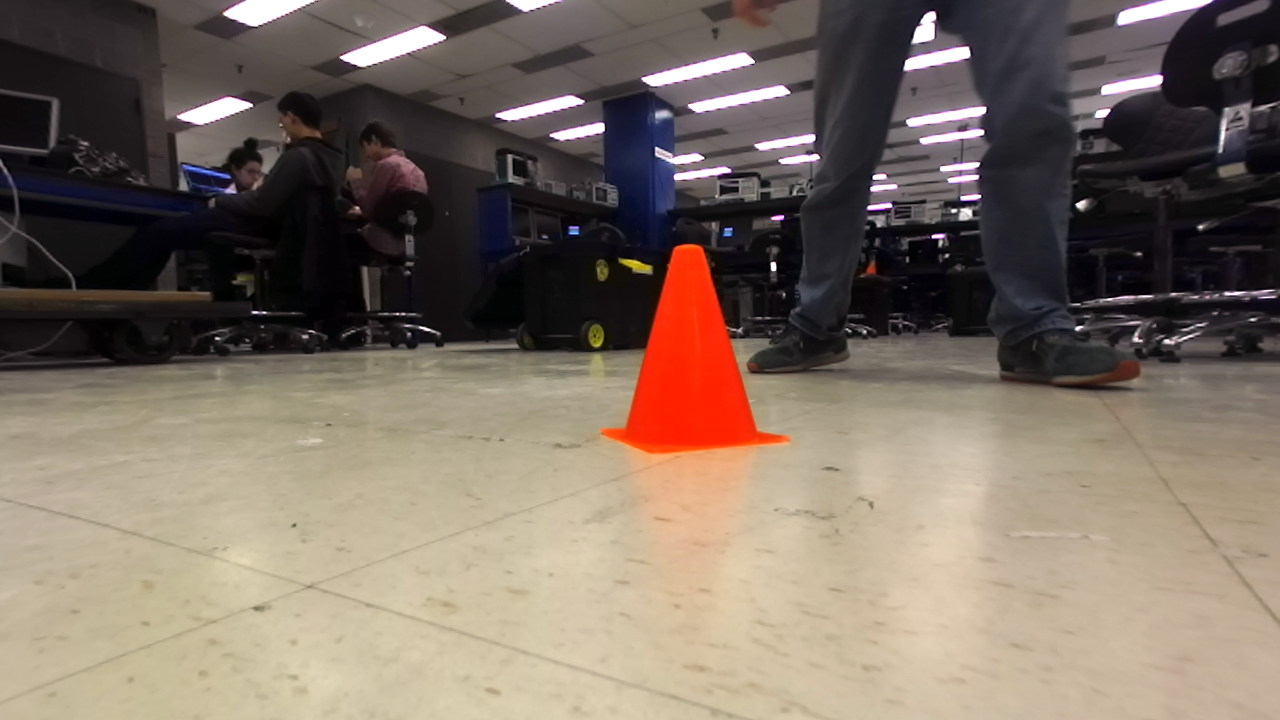
Thresholding
There are two different things that could be looked for when trying to locate the cone in this image - shape, and color. Our implementation chose to discard shape, and classify cones exclusively by color. In order to do this, the color of the cone must be measured.
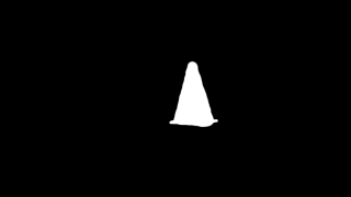
A video of a static cone was recorded, with the lighting conditions varying. This aimed to capture all the possible colors that the cone could appear as. As the cone did not move within the frame, it was possible to hand-draw a mask over a single frame, to label where the cone is. Samples can then be taken from all the pixels under the mask, for every frame, yielding a large dataset of shades of cone-orange.
Using this data, there are a number of common options for building a classifier:
- choose upper and lower bounds for R, G, and B
- choose upper and lower bounds for H, S, and L
- find a small set of planar classifiers - a set of planes which contain the region of color-space holding orange colors. This generalizes the above two options
- Attempt to use machine learning to come up with non-linear classifiers
A little more thought revealed a much simpler option - building a lookup table from color to orangeness. The following plots show the collected color data as voxels, where a voxel is filled if at least one of the samples of the cone falls inside it.
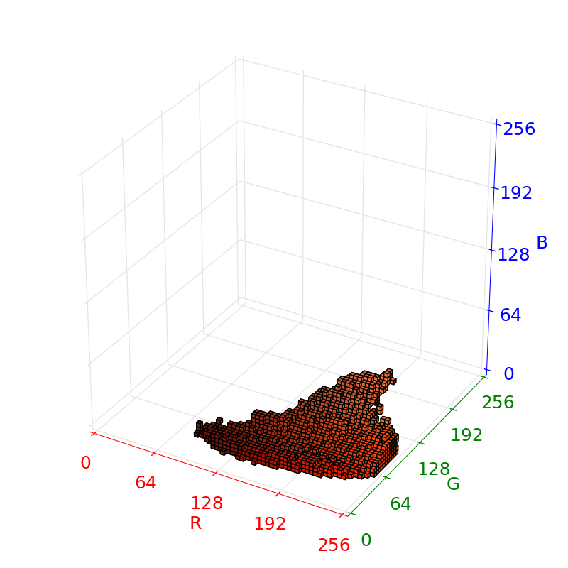
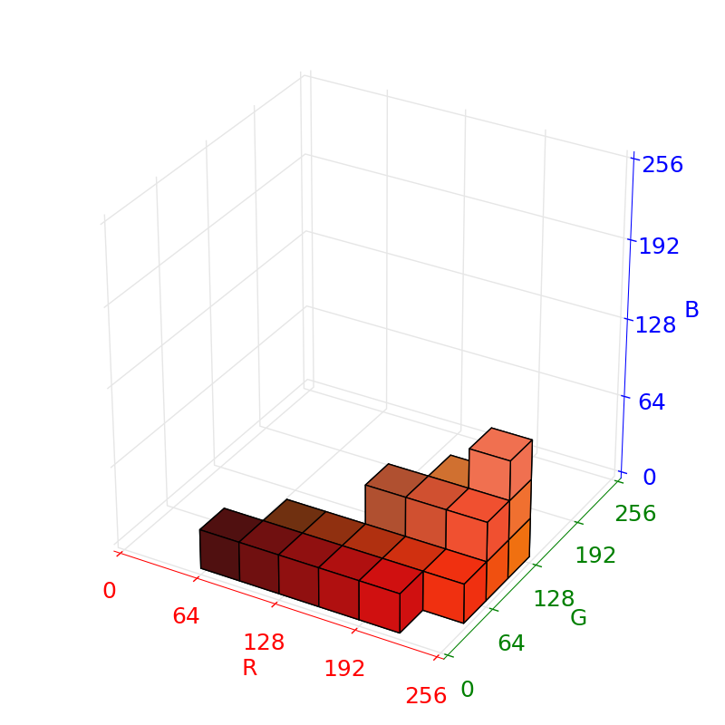
Some thought must be put into choosing voxel sizes: too small, and the size of the lookup table might cause cache invalidation performance issues, and unless a very large amount of data is recorded, the tables will be sparse; too large, and the classifier will group non-orange colors with orange. We settled on a total of voxels.
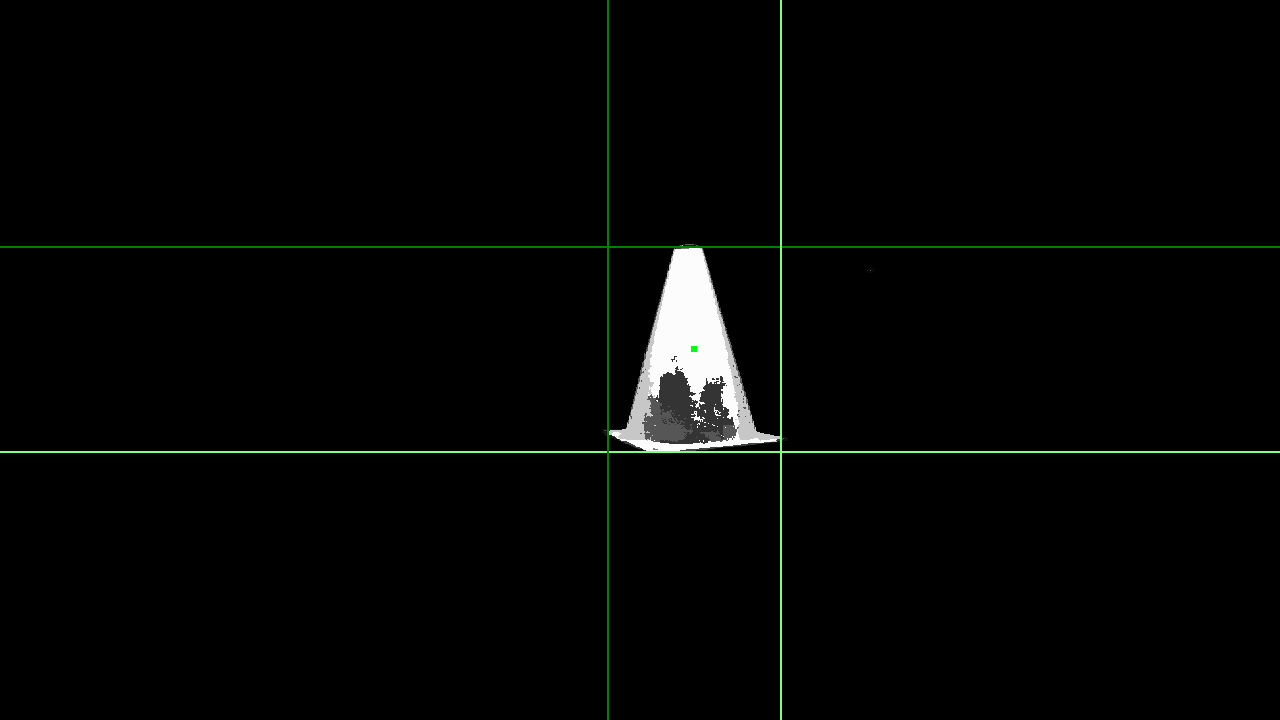
The output of the thresholder is the result of taking every pixel in the raw image, and looking up how many times that region of pixels occurred in the calibration sample. The result is returned as a grayscale image, with white representing the colors seen most in calibration, and black representing colors never seen in calibration.
Blob Detection
The cone_locator node reads the cone_mask topic published by the cone_thresholder node and finds the cone in the mask. It does this using scipy’s labeling feature. The cone_mask is first turned into a binary image by thresholding it at 127/255. This throws away potentially useful information, but is a simplification which allows for using simple labeling. It then uses scipy.ndimage.measurements.label to find the unique connected blobs which are white in the binary image. These are the objects which are cone-colored, like the cone, other far away cones of other teams, and our shoes. It selects the largest cone by visual area and finds the bounding box of that. It publishes the location of the largest such blob to a cone topic of type CameraObjectsStamped.
The definition of the message types is as follows:
CameraObjectsStamped:
- Header header
- CameraObject[] objects
CameraObject:
- string label
- geometry_msgs/Point center
- geometry_msgs/Vector3 size
Extracting Spatial Information
The behaviour of a camera can be described with a rectangular projection matrix. This transforms homogeneous coordinates from the world space to the image plane. ROS sends this information by default alongside any image messages - the topic /camera_info, of type CameraInfo. The property of interest is CameraInfo.P. Interpreted as a 3 × 4 matrix, this satisfies the equation below
Where is the position in world space, and is the position in image space. The constant encapsulates the rules for homogeneous transformations.
This can first be used to convert the pixel widths of the cone into a depth, using known information about the size of the cone, , . We start by considering two points in 3D which are the right distance apart, and finding where they project to:
For our matrix, it turns out that , so this simplifies to:
Note that this equation is overconstrained - there are essentially two equations but only one unknown. We choose to pick the solution that predicts the nearer cone, which we’ll call , since this deals better with cones partially occluded by the edge of the image.
By combining the projection equation, which is underconstrained, with a constraint that , the 3D position can be found by solving a simple matrix equation:
Mitigating Input Image Latency
During the implementation of our team’s computer vision algorithms, we noticed that our robot had a significant perception delay. For the 1st implementation of our vision code, our robot could see and track the cone, but would would take up to half a second to adjust to changes in position of the cone. To debug this perception latency issue, we wrote a node (shown below) that measured the message propagation delay between a set of 2 nodes in our control algorithm.
To achieve this, our C++ latency measuring node listens in on packet_entered_node and packet_left_node Header messages that every node in our system emits directly after serializing an input packet or broadcasting an output message (respectively). The header messages for packet_entered_node, packet_left_node, and the output packet of the node are carbon copy clones of the header message included in the input to our processing node. This allows us to debug latency issues throughout our entire node tree.
By feeding the packet_entered_node and packet_left_node Headers to our node latency calculator, our latency calculator node outputs propagation_delay and upstream_delay statistics in String form on a unique, human-readable topic. For the example graph above, propagation_delay is the delay in ms between a packet entering /lab4/cone_thresholder and entering /lab4/cone_locator, upstream_delay is the age in ms of the packet that has entered /lab4/cone_thresholder, and the output topic is /lab4a/cone_thresholder/debug/processing_lag.
Using this new node type, we were able to diagnose our issues with input latency by connecting this node to multiple configurations of upstream and downstream nodes. Is it turns out, /lab4/cone_thresholder and /lab4/cone_locator each take about 45ms to process image data. However, /camera/zed/zed_wrapper_node outputs images that are 300ms old! Therefore, our perception delays seemed to come from the Zed camera and not our image processing code. Using this information we were able to reduce our input delay to an acceptable level by reducing the output resolution of the Zed camera.
Control
Two control schema were used over the course of the lab. The first was image-based visual servoing. Here, the results of the cone detector’s bounding box were directly fed as input to the controller. This was applied to the first part of the lab with the objective of parking the racecar in front of the cone. The bounding box was fed directly into a p-controller with a hard-coded setpoint for the bounding box location and size, resulting in the desired behavior.
The second was pose-based visual servoing. Here, the cone detectors’ results were first fed into an intermediate pose estimation node before using the cone pose estimate as input to the p-controller. This controller was applied to the second part of the lab with the objective of swerving the racecar around a line of cones in a serpentine. This p-control was used while the cone was in sight of the camera, and the car followed a fixed-radius turn when the cone was not in sight.
Open Source Contributions
- Condense layout of RQT node window
 - Fix a remote code execution vulnerability in
 cv_bridge - Fix malformed packets with python 3
 - Fix a memory leak
 - Diagnosed a segmentation fault.