Lab 5 Writeup
There were three primary goals for this lab. These were:
- Mapping: Collect
Odometry,LaserScan, andTransformdata with the racecar, in order to create a map on the VM. Do this using existing tools within the ros infrastructure - Localization: Using the pre-recorded map information, create a particle filter to find the pose of the racecar using realtime
OdometryandLaserScandata. - Control: Given a preset path, design a controller which causes the robot to follow the path.
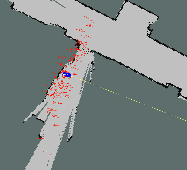
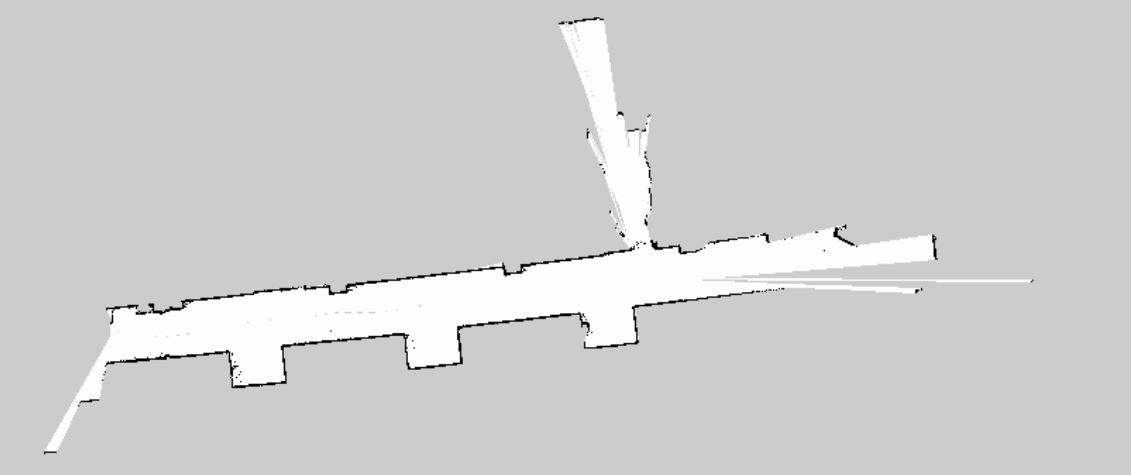
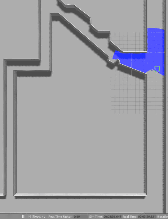
Table of Contents
Mapping
A handful of ros bag files were recorded of the robot driving through some MIT corridors. A launch file was then used to play back these bags alongside a node from one of ROS’ mapping packages. Two tools were tried - hector_slam, and gmapping.
Despite attempts at tuning parameters, we encountered significant problems with the performance of gmapping, which would update its map too infrequently for it to successfully match scans. We worked around this by simulating everything at 1/20th real-time, using a-r 0.05 argument to the rosbag node. This gave gmapping plenty of time to catch up.
hector_slam was able to produce a map of similar quality to gmapping, but could do so without the aid of a slower bag.
Both mapping strategies had a flaw where they would create walls behind the car. This was discovered to be because the laser scanner was detecting parts of the car. This was fixed by narrowing the range of angles that the laser would scan.
Localization
To achieve localization we implemented a particle filter to combine odometry and laser scan information. Particles were tracked as 2-dimensional poses consisting of x, y, and theta. The motion update step occurred each time odometry information was received, producing one particle from each existing particle based on the motion dynamics specified by the odometry and perturbed by a covariance we estimated. The sensor update occurred each time laser scan information was received, using Bresenham ray-tracing to estimate the likelihood of each particle given the map produced by the SLAM algorithms in part 1, resampling the particles based on these weights to improve the estimates.
Motion estimates
The vesc nodes publish an Odometry message on vesc/odom containing the instantaneous angular and linear velocities of the base_link frame. We can integrate these to get an estimate of position.
It should also publish the covariance matrix of these velocities, but it does not. We therefore make some assumptions to calculate this ourselves. We assumed:
Where is the steering angle. These values can be propagated through the equations of dynamics to produce covariance estimates for , the results for which can be seen in this pull request.
Once we have the velocities and their covariances, we are able to take samples from a multivariate normal distribution:
We sample our velocities from this distribution, then use an approach considering the angle half-way through the motion in order to integrate these velocities into poses:
Instead of using , we estimate it as the mean change in time between samples. This is because we are attempting to estimate the time until the next odometry reading, which we do not expect to be significantly larger or smaller than our prior based on the variance of the prior time difference.
Sensor weighting
To implement sensor update, since we were initially not using the map packages in AMCL we must implement raytracing to find the expected range of a sensor reading. To do so, we began with Bresenham’s line algorithm. Given two grid points, the line algorithm returns most of the grid cells that the line connecting the two grid points’ centers passes through. However, since it does not return all of the points, a modified version was used.
In order to return the weights associated with each particle, we approximated the probability densities of the error with a Gaussian with mean 0. A standard deviation was picked that offered reasonable output probabilities.
Once we discovered that using Python code would be far too slow, the raytracing implementation was redone in C and modeled after the AMCL packages. As discussed below, we performed the raytracing component of the sensor update in C and used its output with the ctypes library.
Control
Robust Path Following Using P-control
Following the specifications for Lab 5B, we implemented a proportional controller that follows a path of waypoints based on localization information available to the robot. This controller is passed a message of type nav_msgs/Path containing a set of global waypoints for the robot to traverse in order. However, since we expect that our higher level path-planning navigation system will take some time to run, we designed our path follower node to seamlessly deal with path messages that arrive sporadically or delayed. To the left, you can see a GIF of this path-following node in action using odometry information from Gazebo internals.
To accomplish this, our path follower node maintains an internal state consisting of current_path and next_waypoint_index. Using these two internal state variables, the path follower node can determine when a received path message is new and also which waypoint the robot should proceed to first along the waypoint path.
This last part is especially important if the robot is traveling at speed when a new path arrives at the path follower node. Under this condition, the robot is very likely to receive a path where the first waypoint is already behind the robot and should therefore be ignored.
Testing Path Following Using Gazebo
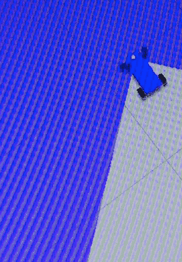
To test our path planner, we wanted to be able to run our path planning software in the Gazebo simulation environment. However, since the stock racecar_simulator code does not support odometry output for the robot, we tried pulling in patch a05d4c8 from upstream. However, this odometry patch was a breaking change caused by overconstraints caused by the addition to a libgazebo_ros_planar_move motion controller to the existing Ackermann based control system. This control contention caused some pretty hilarious consequences (see the GIF on the left, taking careful note of the position of the car’s font wheels).
To fix this problem, we reverted the upstream commit a05d4c8 and created an odometry node that takes in information from Gazebo internals and outputs odometry information on topic /odom (see figure below). Using this new node, odometry now functions as expected in Gazebo, allowing us to create a path follower that allows the robot to traverse the entire tunnel system in simulation.
Writing performant code in python
Vectorization with numpy
When using a for loops in python with a very simple body, the overhead of the looping can become significant compared to the operation inside. Consider the following code:
for p in particles:
    for angle in angles:
        x = p.x + math.sin(angle)
        y = p.y + math.cos(angle)
In this, the workings of the for loop end up doing a function call to __iter__ every iteration. Additionally, we do an attribute lookup on math for every iteration of our loop. Both of these operations can be eliminated by rewriting the code as the following
xs = particles[...,np.newaxis].x + np.sin(angles)
ys = particles[...,np.newaxis].y + np.cos(angles)
Regardless of the size of our dataset, these lines run exactly once each, so we needn’t worry about repeated overhead of function lookup. The for loops are now hidden away in the C code behind numpy, which is highly optimized.
Delegating to C code
Sadly, not all code is easily vectorizable. Generally, if you don’t know the number of loops you need in advance, you’ll have a hard time doing so.
An example of this is raycasting, where you want to walk along a ray until you hit a wall. This is a big part of our sensor update algorithm, but seemed immune to vectorization - we needed a different strategy.
We settled on rewriting this code “closer to the metal”. There are a number of ways which this can be done:
- Using the C API provided by CPython, which provides function for C code to read and write python objects
- powerful
- steep learning curve
- Using Cython, which converts a slightly modified version of python to C code.
- very easy to create
pyxfiles from existing python code - interacts well with numpy
- not well-supported for building with catkin
- very easy to create
- Build a simple shared object file in C, and use
ctypeswithin python to call into it- messier python code
- very easy to build with catkin
- C code does not need to know about python
We settled on the last option, which results in C code like:
void calc_line(int8_t* map, size_t xlen, size_t ylen, size_t sx, size_t sy, size_t *tx, size_t *ty) { ... }
And the somewhat messy python wrapper to call this function from python:
from ctypes import *
from numpy.ctypeslib import ndpointer

calc_line_c = cdll.LoadLibrary('libmonte_carlo_localization.so').calc_line
calc_line_c.restype = None
calc_line_c.argtypes = [ndpointer(c_int8, flags="C_CONTIGUOUS"), c_size_t, c_size_t, c_size_t, c_size_t, POINTER(c_size_t), POINTER(c_size_t)]

def calc_line(map, start, target):
	tx = c_size_t(target[0])
	ty = c_size_t(target[1])
	xlen, ylen = map.grid.shape
	calc_line_c(map.grid, xlen, ylen, start[0], start[1], tx, ty)
	return ty.value, tx.value
Profiling
The results of the above optimizations are summarized below
| Approach | Time to process a scan with 100 rays for 20 particles |
|---|---|
| Original | 10s |
| Vectorized with numpy | 3.8s |
| Bottleneck ported to C | 2.4s |
| Both of the above | 0.13s |
Open source contributions
- Related to the
rosbagAPI:- ros/ros_comm#769
- ros/ros_comm#772
- ros/ros_comm#777
- Diagnosis and patches for bugs related to
rospy.Durationarithmetic- ros/genpy#48
- ros/genpy#49
- ros/genpy#50
- ros/genpy#52
- ros/genpy#53
- ros/genpy#54
- ros/ros_comm#781
- ros/ros_comm#783
- Fixes to the RSS2016 codebase
- https://github.mit.edu/racecar/vesc/pull/3
- https://github.mit.edu/racecar/racecar_simulator/pull/6
- https://github.mit.edu/racecar/racecar_simulator/pull/7
- https://github.mit.edu/racecar/racecar_simulator/pull/9
- https://github.mit.edu/racecar/racecar_simulator/pull/10
- https://github.mit.edu/racecar/racecar_simulator/pull/11
- https://github.mit.edu/racecar/racecar_simulator/pull/13
- https://github.mit.edu/racecar/racecar_simulator/pull/14
- https://github.mit.edu/racecar/racecar/pull/15