Lab 6 Writeup
Our goal for this lab was to create a path planning algorithm that could navigate the robot down a corridor whilst avoiding obstacles. To achieve this, our team implemented a Rapidly-exploring Random Tree (RRT) algorithm and made modifications to our previous path following algorithm. Our final results were that we were able to drive down a hallway in the Gazebo simulator using a pre-recorded map-file.
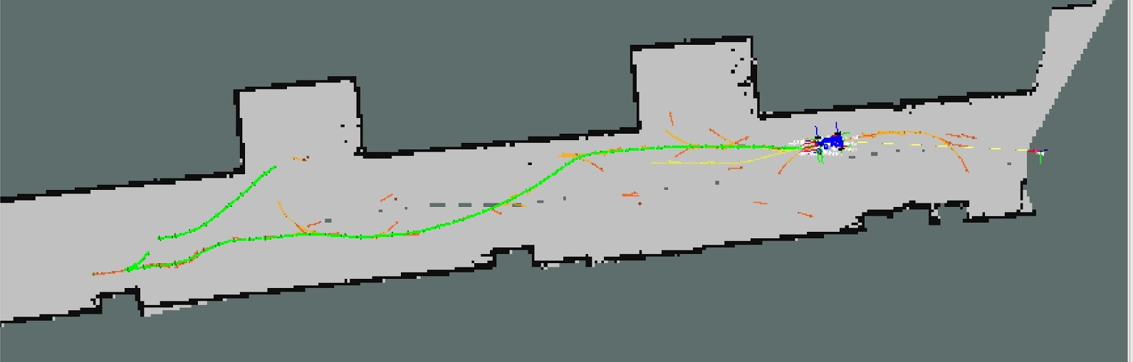
Table of Contents
Selecting a Mapping Strategy
In order to effectively find paths, the robot needs a model of its surroundings in which to plan. This entails both knowledge of where obstacles are located in the world and where the robot is in the world. We investigated two different potential alternatives for this. The first was a divided approach, which localized using a known map and the AMCL library and created an ad-hoc local map based on the laser scans and the transform determined by AMCL. The alternative was simply to use hector-slam to both create a map and localize within it.
The first approach has the advantage of being less computationally expensive, because not all of the functions of SLAM were actually required for the task. However, it is more complicated to implement than simply using an integrated SLAM package. Conversely, SLAM involves more computation than is necessary but required only using a single pre-implemented package. On testing hector-slam on the robot, we found that it was able to run sufficiently fast despite the extra computation, so we went with the second option.
Selecting a Pathfinding Algorithm
The team looked over the pathfinding algorithms covered in class in order to select one to implement. The choices were potential fields, probabilistic roadmap (PRM), and rapidly-expanding random trees (RRT). In an ideal universe we would have created implementation stubs for each of these and evaluated which one worked best in simulation in order to pick one for the final race. In the non-ideal universe where we have one week to write implementation code while balancing other classes, we had to make a choice of one algorithm to implement.
In order to do this, we judged the algorithms on ease of implementation as well as the completeness of the algorithm. Along these metrics, potential fields seemed to be the easiest to implement, followed by the RRT and PRM being somewhat equivalent in difficulty. As for completeness, potential fields seemed to be the worst due to the possibility of getting stuck in a concave obstacle between the car and the goal. PRM is worse than RRT because it cannot handle dynamic obstacles as well. As a result, we picked the RRT to implement because we expected it to result in the most complete solution.
Path planning with RRTs
There are four key parts to a Rapidly-expanding Random Tree planner:
sample- A method to sample a point to trydistance- A metric for determining the distance or cost between a visited point and an unvisited pointextend- A rule for extending towards a new location from an existing onedone- A condition for when to stop
We started by writing the core algorithm that wraps these four operations as an abstract class (using pythons abc module), which allowed us to swap out these functions without rewriting the entire RRT each time.
For the purpose of testing our algorithm, we reused the map file from lab5 that we recorded of one of the RLE corridors, and added some extra dark rectangles that correspond to the size of a cone. These were arranged mostly randomly, but we made sure to include a pathological case of a wall of cones to test the algorithm
A simple RRT
For a simple RRT, we filled out these key parts as:
sample:- With a chance, choose the goal location
- Otherwise, choose a random point in the bounding box circumscribed around a circle 1.5× the diameter of the smallest circle passing through the start and end points of the planner, as in the below interactive diagram.
distance- Use the cartesian distance metric,extend- Linear interpolate up to 0.5m towards the goal, stopping early if the line hits a walldone- Stop if the distance to the goal is less than 0.1m
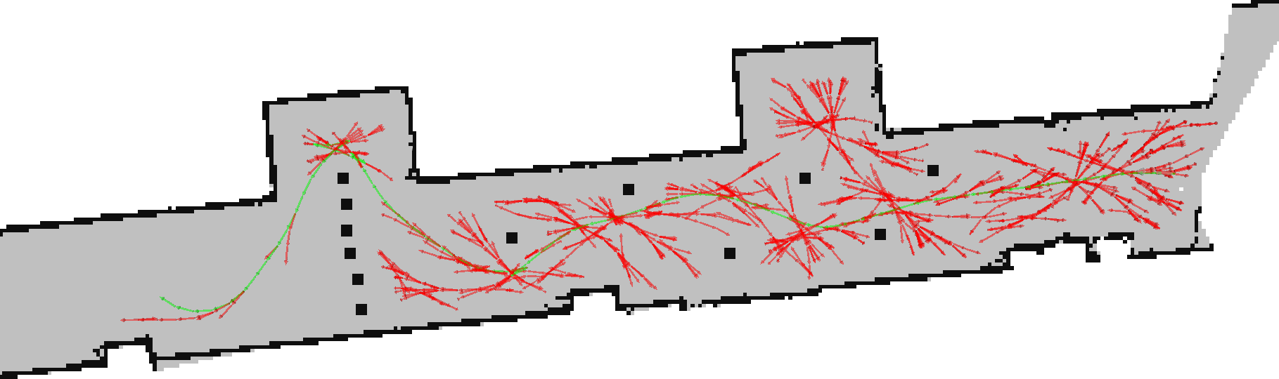
The result of running this algorithm is shown below:
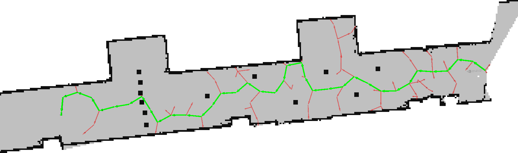
The red arrows show the attempted paths, and the green chain of arrows the solution path. Note that the solution found cuts through the wall, because we are modelling the car as a point, and not doing full collision detection. Also, some of the corners this generates are very sharp, which is not so viable for an ackermann-steered car
Modelling the car more accurately
sample- With a chance, choose the goal location
- With a chance, choose a random free point from the bounding box between the goal and the nearest point on the tree so far, defined in the same way as in the other RRT
- Otherwise, choose a random free point using the same rules as before
distanceReturn the length of the shortest circular arc connecting the existing point to the new one. If such an arc would be too tight for the car to follow, returnextend- Spherically interpolate up to 0.25m along the arc found in the distance function, stopping early if any part of the car would be intersecting a walldone- As before
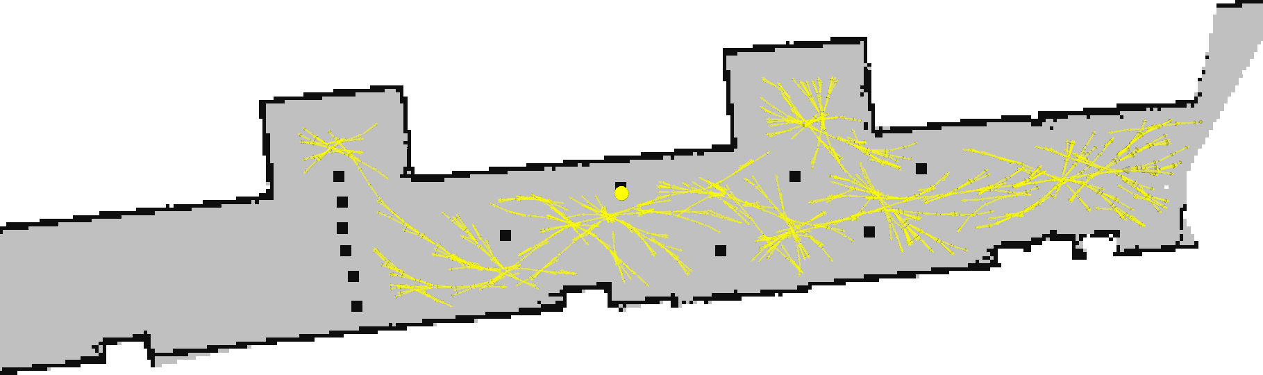
This algorithm takes much more time to run, so we made sure to visualize it as it was running. Here, the yellow dot shows an example of a point that is being considered from the sample phase.
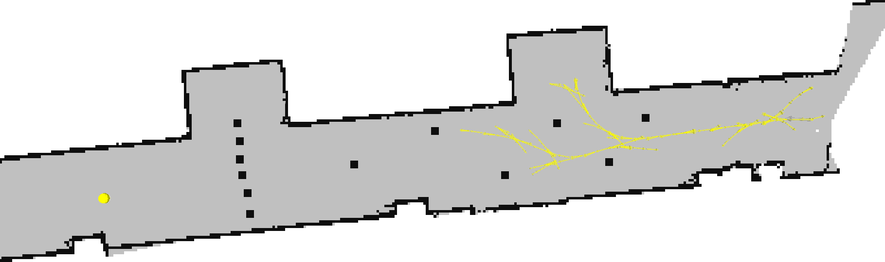 Immediately, we can see that the paths we are finding respect the constraints imposed by an ackermann trajectory.
 After a while longer, the tree expands into most of the large empty regions.
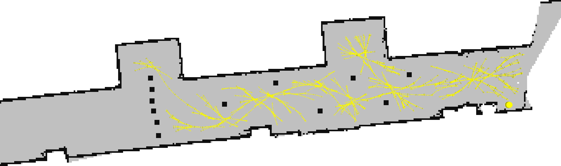 We get stuck against the wall of cones for quite some time, as we require a 3-point turn to turn around the top of the wall.
 40 minutes later, a viable path is found.
Updating the path_follower for usage with RRT
For optimal usage of the RRT, our path_follower node needed to be improved in the following ways:
- The path_follower node should be able to report the status of execution of the current path to the RRT.
- It should also be able to drive backwards since RRTs can output paths that require the robot to reverse.
- (Optional) the
path_followershould be able to tell the RRT when something bad (such as an E-stop event) has happened and that the RRT should forcibly replan a path from the car’s current location.
To allow for our RRT algorithm to create optimal paths, we assumed that our RRT would only give a small portion of the path to execute at a time. This way, our RRT could use the time that the robot is executing the path to optimize the remaining portion of the path. Under this design choice, allowing our path_follower to report its execution progress was simple. The path_follower node simply published the topic /lab6/path_follower/execution/complete and sent a Header message whenever the node had finished executing the given path.